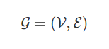
Figure convolution network definition and simple example
Many important data sets in today's world come in the form of diagrams or networks: social networks, knowledge charts, protein interaction networks, the World Wide Web, and more. Until recently, however, people began to focus on the possibility of generalizing neural network models to handle such structured data sets.
At present, some of them have achieved very good results in the professional field. The best results before this are obtained by the kernel-based method, the graph theory-based regularization method or other methods.
OutlineA brief introduction to the neural network diagram model
Spectral Convolution and Graph Convolution Networks (GCNs)
Demo: Graph embedding with a simple first-order GCN model
Think of GCNs as a micro-generalization of the Weisfeiler-Lehman algorithm
If you are already familiar with GCNs and their associated methods, you can skip to the "GCNs Part III: Embedding Karate Club Network" section.
How powerful is the graph convolution network?
Recent literatureGeneralizing mature neural models (such as RNN or CNN) to process arbitrary structural graphs is a challenging problem. Some recent papers have introduced proprietary architectures for specific problems. There are also convolution maps built on known spectral theory.
To define the parametric filters used in the multi-layer neural network model, similar to the "classic" CNN we know and use.
More recent research has focused on narrowing the gap between fast heuristics and slow heuristics, but with a more solid theoretical approach to spectrum. Defferrard et al. (NIPS 2016, https://arxiv.org/abs/1606.09375) used a Chebyshev polynomial with free parameters learned in a neural network model, and an approximate smoothing filter was obtained in the spectral domain. They have also achieved convincing results in conventional areas such as MNIST, approaching the results obtained from simple two-dimensional CNN models.
In Kipf & Welling's article, we took a similar approach, starting with the spectral convolutional framework, but with some simplifications (we'll discuss the details later), which in many cases is significantly faster The training time has been improved and the accuracy is obtained. The best classification results are obtained in the test of many benchmark data sets.
GCNs Part I: Definitions
Currently, most graph neural network models have a common architecture. These models are collectively referred to herein as Graph Convolu TIonal Networks (GCNs). It is called convolution because the filter parameters are usually shared at all locations in the graph (or a subset thereof, see Duvenaud et al., 2015, published in NIPS).
The goal of these models is to learn a function from the signals or features on the graph.
And take it as input:
The feature description x_i of each node i is summarized as a feature matrix X of N * D (N: number of nodes, D: number of input features)
A representative description of the graph structure in the form of a matrix, usually represented by an adjacency matrix A (or some other related function)
A node-level output Z (N * F feature matrix, where F is the number of output features per node) is then generated. Graph-level output can be modeled by introducing some form of pooling operation.
Then each neural network layer can be written as a nonlinear function:

Where H^(0)= X, H^(L)= Z (or z is output as a graph), and L is the number of layers. The specificity of the model is only manifested in the choice and parameterization of the function f( , ).
GCNs Part II: A simple example
Let's take the following simple hierarchical propagation rules as an example:
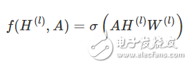
Where W(l) is the weight matrix of the lth neural network layer and σ() is a nonlinear activation function such as ReLU. Although this model is simple, its function is quite powerful (we will talk about it later).
But first we need to clarify two limitations of the model: multiplication with A means that for each node is the sum of the eigenvectors of all adjacent nodes without including the node itself (unless there is a self-loop in the figure) . We can "solve" this problem by enforcing self-looping in the graph - just add the identity matrix to A.
The second limitation is that A is usually not normalized, so multiplying A will completely change the distribution of the eigenvectors (we can understand this by looking at the eigenvalues ​​of A). Normalize A so that the sum of all rows is 1, ie D^-1 A, where D is the diagonal node degree matrix, which avoids this problem. After normalization, multiplying by D^-1 A is equivalent to taking the average of the features of adjacent nodes. Symmetric normalization can be used in practical applications, such as D^-1/2 AD^-1/2 (not just the average of adjacent nodes), and the dynamics of the model become more interesting. Combining these two techniques, we basically got the propagation rules described in the Kipf&Welling article:

Where A = A + I, I is the identity matrix, and D is the diagonal node degree matrix of A.
In the next section, we'll take a closer look at how this model works on a very simple example diagram: Zachary's Karate Club Network.
GCNs Part III: Embedding the Karate Club Network
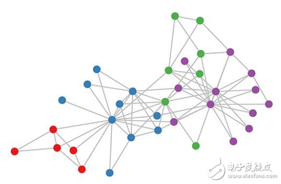
The color of the karate club map represents a community obtained through modular clustering (for details, see the article published by Brandes et al. in 2008).
Let's take a look at how our GCN model works on the famous graph dataset: Zachary's Karate Club network (see above).
We used a 3-layer GCN with random initialization weights. Now, even before we train the weights, we simply insert the adjacency matrix of the graph and X = I (ie the identity matrix, because we don't have any node features) into the model. The three-layer GCN performs three propagation steps during forward transfer and effectively convolves the third-order neighborhood of each node (all nodes reach a three-level "jump"). It is worth noting that the model generates an embedding for these nodes that is very similar to the community structure of the graph (see figure below). So far, we have initialized the weights completely randomly and have not done any training yet.
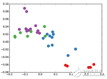
Embedding of GCN nodes in the karate club network (random weights).
This seems a bit surprising. A recent model called DeepWalk (Perozzi et al., 2014, published at KDD https://arxiv.org/abs/1403.6652) shows that they can achieve similar embedding in complex unsupervised training. So how can we get this kind of embedding just by using our untrained simple GCN model?
We can get some inspiration by considering the GCN model as a generalized differentiable version of the well-known Weisfeiler-Lehman algorithm in graph theory. The Weisfeiler-Lehman algorithm is one-dimensional and works as follows:
For all nodes
Solving the feature {h_vj} of the neighboring node {vj}
Update the node feature by h_viâ†hash(Σj h_vj), where the hash (ideally) is a single-shot hash function
Repeat k steps or until the function converges.
In practical applications, the Weisfeiler-Lehman algorithm can assign a unique set of features to most graphs. This means that each node is assigned a unique feature that describes the role of the node in the graph. But this is not applicable to highly regular graphs like grids, chains, etc. For most irregular graphs, feature assignments can be used to check the isomorphism of the graph (ie, from the nodes to see if the two graphs are the same).
Go back to our layer convolution layer propagation rules (represented in vector form):
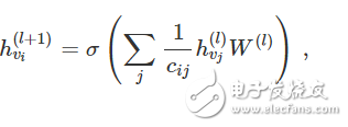
Where j is the neighbor of v_i. C_ij is the normalized constant of the edges (v_i, v_j) generated using the symmetric normalized adjacency matrix D-1/2 A D-1/2 in our GCN model. We can interpret this propagation rule as a differentiable and parameterized (for W(l)) variant of the hash function used in the original Weisfeiler-Lehman algorithm. If we now choose an appropriate, non-linear matrix and initialize its random weights to make it orthogonal, then this update rule will become stable in practical applications (this is also due to the c_ij in normalization). usage of). We came to the very insightful conclusion that we got a very meaningful smooth embedding, in which the distance can be used to represent the (not) similarity of the local graph structure!
Part IV of GCNs: Semi-supervised learning
Since everything in our model is distinguishable and parameterizable, you can add tags that you can use to train your model and see how the embes react. We can use the semi-supervised learning algorithm of GCN introduced in the Kipf&Welling article. We only need to mark one node per class/common (the node highlighted in the video below) and then start several iterations of training:
Semi-supervised classification with GCNs: 300 iterations of training with a single label for each class to obtain the dynamics of the hidden space. Highlight the marker node.
Note that the model will directly generate a two-dimensional hidden space for instant visualization. We observed that the three-layer GCN model attempts to linearly separate these classes (with only one tag instance). This result is compelling because the model does not have any characterization of the receiving node. At the same time, the model can also provide initial node features, so the current best classification results can be obtained on a large number of datasets, which is the result of the experiments we described in the article.
in conclusion
Research on this field is just getting started. In the past few months, the field has gained encouraging development, but so far we may have just captured the appearance of these models. How to study the specific types of problems in graph theory, such as learning on orientation maps or diagrams, and how to use the embedded graphs to complete the next task, remains to be further explored. The content of this article is by no means exhaustive, and I hope that there will be more interesting applications and extensions in the near future.
With 15+ years manufacturing experience for Portable Power.
Supply various portable charger for iPhone, Airpods, laptop, radio-controlled aircraft ,laptop, car and medical device mobile device, ect.
From the original ordinary portable power source to Wireless Power Bank, Green Energy Solar Power Bank, Magnetic Mobile Power, Portable Power Stations and other products continue to innovate.
Avoiding your devices run out of charge, Portable Chargers to keep your mobile device going.
We help 200+ customers create a custom mobile power bank design for various industries.
Wireless Earphones,Wireless Headphones,Best Wireless Headphones,Best Bluetooth Earphones
TOPNOTCH INTERNATIONAL GROUP LIMITED , https://www.micbluetooth.com